12.5. From text to data

To build intuition for how we turn text into data, we will work mostly from the text-as-data approach. But, many of the steps are similar for other applications, though some of our more simplifying assumptions (such as Bag of Words, as decribed below) may not work if we’re trying to get languages to speak in a manner that sounds human. For now, however, this is the overall process for working with text data of any kind:

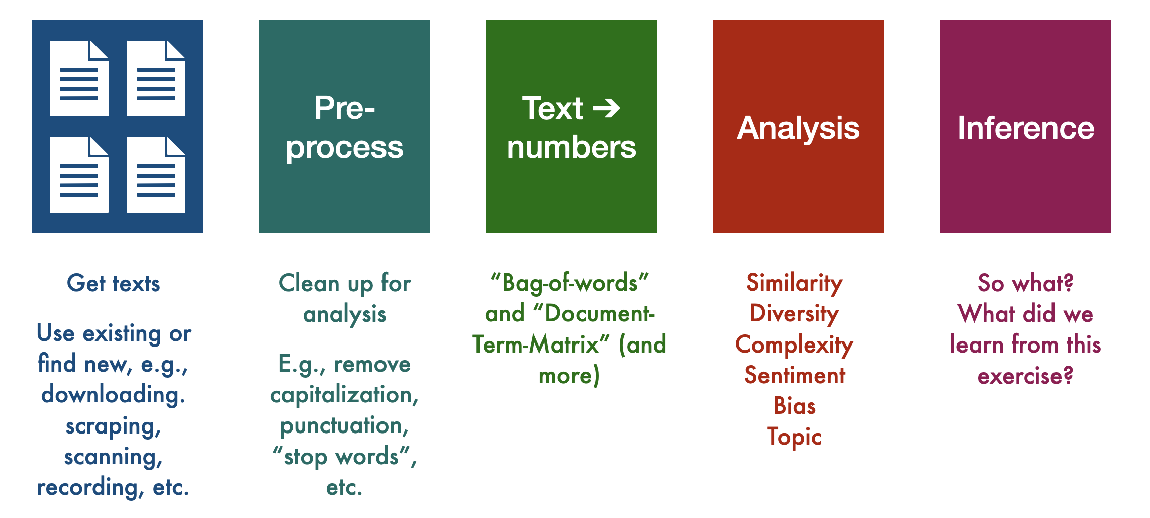
Fig. 12.6 General order of operations for conducting a text-as-data analysis

Useful vocabulary

We will shortly work through a real (albeit simple) example from start to finish to more closely inspect each step. Before we do that, howev er, we will also need some vocabulary:

Our data

• Corpus: a collection of documents (plural: corpora)

• Document: a collection of texts (corpora > corpus > documents > doc1, doc2, etc.)

For example, if I wanted to study how the New York Times covered the Obama administration, my corpus might be all “NYT articles between January 20, 2009 and January 20, 2017 that contain the word “Obama” at least once. My documents would likely be each article in our corpus.

Alternatively, if I were doing an analysis of the sentiment of Twitter users towards Elon Musk after his takeover of Twitter, I might have a corpus that includes a certain number of tweets with the words “Elon” or “Musk” from perhaps the first month of his takeover as well as from the month prior his takeover. In this case, our documents would each be one tweet.

Tokenizing

We need to chop up each document into units that the computer can make sense of (this is the simplest version; there are techniques where we chop text into sentences, paragraphs, or not at all, and while that can provide more accurate analyses (though not necessarily), it quickly becomes very computationally intensive).

• Token: a sequence of characters in a document that are grouped together as a useful unit; e.g., a word or number (in English, this is often whitespace-based; i.e., we say a token ends when there is a space between letters. This is not always perfect, but it’s a simple and reasonably effective start).

• Type: the number of unique tokens in a document (so, the number of different words in a doc)

• Tokenization: the process of actually chopping up our text based on a rule, such as look for whitespace and cut there

Cleaning and standardization

Depending on our research goals, we will likely want to do some kind of cleaning and standardization of our data. This often requires making decisions about:

• Stop words: commonly used words, such as “the”, “and”, “of”, etc., that we may want to exclude from our analysis

• Punctuation & capitalization: if we simply cut up documents by the presence of whitespace, this means that, for example, the words run, Run, and run., and run, would all be stored as unique types. This might be useful for us, but more than likely it is a distraction and unnecessary complication if what we really want to understand is how often the word run is used. Thus, we may want to remove capitalization and punctuation from our text.

• Stemming: a technique where we reduce words to their root or base form. Most stemmers operate by (rather bluntly) chopping off commonly used prefixes or suffixes from words (e.g., dropping “-ing” or “-ed” from the ends of words). Note that this will not necessarily generate real words. For example, if I wanted to standardize the tokens run and running so they are stored as the same type, a simple stemmer that just lops off “ing” would yield run and runn.

• Lemmatization: a more sophisticated technique by which we normalize words with the use of a vocabulary we provide to the computer. This is generally slower and more computationally intensive – and thus may not be worth it depending on our research goals and size of our dataset – but it would, e.g., generally be better at transforming run, ran, and running (and possibly even runner, though we’d need to inspect and make a decision about whether we want that to count as the same type as run) into simply run.

If these tokenizing, cleaning, and standardizing options are making you nervous – they should! Just as there’s no “right” answer when it comes to choosing how to measure something, or how many variables to put into your linear regression, and so on, there’s no single “right” option when pre-processing your text data (oh gosh, could we build an RL algorithm to explore the strategies, though? Extra credit! (Not really).

In some cases, for example, we might really want to include punctuation – for example if the presence of ! or ? will likely help you better understand the sentiment of your customers or voters. You also will perhaps want to retain capitalization if your data includes a lot of proper nouns that, without capitalization, might be lost as such. For example, if we want to understand sentiments about the company “Apple”, we almost certainly would not want to lowercase it, lest we accidentally collect sentiments around fruit.

While these decisions can at first seem trivial, depending on our work, they can have real implications for our analyses that follow.

Operating on text

We will now do something to our text that will likely incite horror among all literature and language lovers: we are going to (gasp) ingore word order, and then represent each word in a document as a location in the feature space.

• Bag of Words (BoW): One of the simplest and least computationally intense ways to work with text data is to make the seemingly shocking assumption that word order does not matter. This is a simplifying assumption that necessarily causes us to lose some meaning (or even a lot, depending on our text), but also has been demonstrated to still retain (we think) enough “meaning” that we are able to learn a lot about our text even with this assumption.

• Document-Term Matrix (DTM): We are then going to turn our bag of words into a matrix that describes the frequency of tokens within each document in a corpus

Finally, for our analysis in this chapter, we will calculate the similarity of a few example documents in order to evaluate the similarity of texts by two of the most prized writers in human record, William Shakespeare and, of course, Jerry Seinfeld. We will do this using

• Cosine similarity: a metric to calculate the distance between two documents in terms of the cosine of the angle between two vectors projected in a multi-dimensional feature space (really rolls off the tongue, I know!)

To see how this all works, let’s conduct our analysis in Python – onward to the next section!