2.3. Observational studies

To recap: Snow cannot pursue a randomized control trial. So, instead he will need to use observational data. This is a very common scenario. So how can he test his theory? One observation he had was that different areas of London were served by different water companies. In particular, some people got their water from the Lambeth company, and other from the Southwark and Vauxhall (S&V) company. The former supplied London from the Thames well upriver from sewage discharge. The latter did not, and their water was often contaminated with sewage. The map below shows how the companies divided up supply to London residents.

Fig. 2.3 Snow’s second cholera map

Snow showed that households supplied by the S&V company had cholera rates almost ten times those of the Lambeth company:

Supply Area	Number of houses	cholera deaths	deaths per 10,000 houses
S&V	40,046	1,263	315
Lambeth	26,107	98	37
Rest of London	256,423	1,422	59

Importantly, Snow argued that in the area of study, the households did not differ by any other relevant factors—like their average income or health level—that might affect cholera rates. Notice what Snow is claiming: that the two groups of people, one supplied by one company, one supplied by the other, differ only in terms of the treatment. That is, one group (the treated) get the contaminated water, and one group (the control) do not. He has not, and cannot, randomize households to treatment or control; instead, he is arguing that the assignment of water via the water companies is either as if random, or at least not related to other factors (like how rich people are) that might affect the outcome (how sick they get).

Snow’s Legacy

In the short term, Snow was successful in the sense that local authorities kept the pump handle removed in Broad Street, thus saving lives. In the long term, he was also successful: his study has become a classic, and his methods are now widely taught (as we are doing here). Furthermore, his theories about fecal-oral transmission as the route by which cholera spreads in water would ultimately be refined and accepted. In the medium term however, Snow’s theories and methods were not embraced, and he faced considerable opposition in propagating his ideas.

Natural Experiments

Today we sometimes call research designs like Snow’s “natural experiments”. These occur when

assignment to treatment is outside the control of the experimenter but is either as if random, or at least unrelated to other factors (“confounders”) that affect the outcome.

We use the term “confounders” to refer to those “other factors” that affect both

• assignment to treatment (so treatment v control status) and

• outcomes

In observational studies, confounders are a constant threat. We can sometimes show that units in treatment and control are similar on variables we can measure (like health or income) but they still may be dissimilar on variables we cannot easily measure (like political ideology or propensity to lie). These factors are sometimes called “unobserved confounders”. It is easy to find studies that have this potential problem. For example, there is evidence that people who own dogs (treatment) have better heart health (outcome) than those who do not (control). But we can surely think of confounders that affect both the decision to own a dog and heart health – like how much people like to exercise outdoors, or how much free time they have.

Vietnam Draft Lottery

A more modern example of a natural experiment are the studies that use the Vietnam Draft Lottery in the United States. The draft lottery was a way of conscripting young men to go to Vietnam in 1969-70. It was based on the men’s birthdays. To understand how this might work, suppose there were 365 balls in a hat, each with a day of the year written on it. A ball is drawn at random, the day on it is read out, and all American men who are turning 19 on that day must join the military. This is not quite how it operated, but it’s the right intuition.

Why is this useful? Suppose the day drawn is August 5, which means all men turning 19 on August 5 are now drafted. It seems reasonable to suppose that there is no reason that those men differ in any particularly important way from men turning 19 on August 3, August 6, July 10, September 2, and so on. We can follow the men who were drafted as if they were in the treatment group for military service. And we can compare them to those who were not drafted, who are in the control group. If we have an as if randomly selected treatment and control group, we can calculate the causal effect of military service on outcomes like lifetime income, or health. For a famous paper that uses this design see

Angrist, Joshua D. “Lifetime earnings and the Vietnam era draft lottery: evidence from social security administrative records.” The American Economic Review (1990): 313-336.

Ultimately, Angrist finds that military service suppresses later earnings (veterans earn ~15% less).

This lottery design is likely to allow for a much better estimate of the causal effect than just comparing people who choose to serve in the military versus those that don’t: we can imagine all sorts of confounders (like pre-existing fitness, level of patriotism, income level as a child) that would affect both whether you serve and the ultimate outcome (health as a middle-aged adult).

Compliance and Non-compliance

In any experiment (natural or lab) we want the subjects assigned to treatment to take the treatment, and the subjects assigned to control to not take the treatment. We call this compliance. We refer to the opposite situation, where those in the treatment group don’t take the treatment and those in the control group somehow access the treatment, as non-compliance.

It is not hard to think of situations where non-compliance might occur. For example, we can imagine in Snow’s water supply design, some householders supplied by S&V might actually get their drinking water from a Lambeth-supplied pump on the way to work. In the Vietnam lottery case, some draftees might refuse to serve. This could pose a very difficult issue if they are different in other ways to those who were drafted but did serve.

Terminology and Practice in Observational Studies

A common (perhaps annoying) feature of statistics is using different words for the same entity. Here are some important examples you need to know. In an observational study, we have

• an outcome we want to explain: we call this the dependent variable or \(Y\)

• a treatment that does the explaining: we call this the independent variable (or “an” independent variable) or \(X\)

• confounders, \(Z\) which potentially affect both \(Y\) and \(X\)

If, in fact, \(Z\) is a confounder, there may be no causal relationship at all between \(X\) and \(Y\). In this case, we say the (seemingly causal) relationship between \(X\) and \(Y\) is spurious.

Testing Hypotheses

Exactly as in the Snow study, to test hypotheses we need to

compare units with different values on the independent variable (treatment status) in terms of whether this results in different values on their dependent variable (outcomes)

Obviously, the independent variable must vary across cases! We cannot estimate a causal effect of a treatment if everyone is treated (or everyone is not treated). This is similar to our concern above about needing a control group to compare too. In general too, we need variation on the outcomes.

Selecting on the Dependent Variable

Despite the fact that many studies do it, you cannot select on the dependent variable if you want to make causal inferences. Selecting on the dependent variable means

studying only those cases that have the same, particular value as their outcome, typically in terms of what they have in common that might have “caused” that same outcome.

Examples abound (unfortunately):

• in a New York Times story (October 21, 2018) a reporter claimed that “I’ve Interviewed 300 High Achievers About Their Morning Routines. Here’s What I’ve Learned” One of the observations about these people is that they tend to get up early. We cannot know whether this is a causal factor (let alone how important it is) because we only have high achievers in the study. Perhaps low achievers also get up early. Perhaps low achievers get up much earlier.

• it is very common to see stories about what we can learn from long-lived people (you will see headlines like “12 Secrets of People Who’ve Lived to 100”). But these select on the dependent variable—specifically, of being old. We have no idea if the lifestyle tips those old people offer are effective or not, because for all we know, people who die much earlier also did those things. But those people were not in our study.

Survivor Bias

Survivorship bias or Survivor Bias occurs when

a study includes only those units that “survived” (got through, were not made extinct by) a certain process.

Looking only at such units leads to biased inferences, because they are often similarly “special” in some way that affects their outcomes but about which the analyst is unaware. One instance of this is obtaining tips from those who were successful after an extensive interview process. We have no way of knowing if their suggested actions may also have been taken by those who were not successful.

There are more prosaic cases too: for example, people often claim that, say, music was “better in the old days”. They say this based on older music they hear today; but presumably only the best old music survives to be played now—the rest was too bad for anyone to wish to listen to it again. But this is entirely compatible with old music being (much) worse on average than today’s music.

A classic example is “Wald’s bomber”. Wald was a statistician in World War 2. His task was to help the Air Force reinforce armor on their planes to reduce losses from anti-aircraft fire. Consider the following (hypothetical) picture of a typical bomber that successfully returns to base; assume that many planes do not make it back. The red dots are where the planes that returned have sustained damage. The question is: where should extra armor be added to the planes to reduce losses next time?

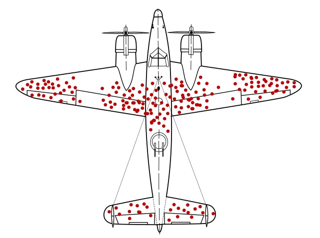
Fig. 2.4 Wald’s bomber (hypothetical) illustration

It is tempting to put armor where the planes were hit. But this is to ignore the key fact that these planes survived these hits. This suggests that hits where the red dots are located are not critical—the planes we observe were hit there, but all made it back. Indeed, it is possible that being hit in places other than the red dots is what caused the other planes not to return. But we don’t get to observe them, because they didn’t survive. So one counter-intuitive lesson is to place armor where the returning planes were not hit.