5.6. Normal distribution

The mean and the variance (the standard deviation squared) are important for characterizing the normal distribution. This is one of the most important distributions in statistics, in part because it is empirically common—a lot of things are normally distributed in nature. But it is also important for the related reason that we have learned a lot about it. That knowledge of the normal facilitates a great deal of statistical reasoning, in terms of assumptions we make and inference we draw.

First, notice that the normal goes by many other names: it is sometimes referred to as a Gaussian distribution (named after Gauss). It is sometimes referred to as the “bell curve”, because it looks like a bell—though this is imprecise and may lead to confusion (a lot of distributions look like a bell).

Second, as noted above, the normal distribution is characterized by its mean and variance (equivalently, its standard deviation). It is unimodal (has one mode) and that mode is equal to its median, which is equal to its mean. So it is symmetric.

The mean tells us the “location” of the normal in terms of its base on the $x$-axis. The standard deviation tells us how spread out it is around that mean. In statistics, when describing the normal, we often use the Greek letter “mu” ($\mu$) to stand in for the mean; and we use “sigma” ($\sigma$) for the standard deviation. We write “sigma squared” (${\sigma }^2$) for the variance.

Though you don’t need to know this for the course, here is the formula for the normal distribution. See if you can see the mean and standard deviation in it:

$$f(x)=\frac{1}{\sigma \sqrt{2\pi }}\exp (-\frac{1}{2}{\left(\frac{x-\mu }{\sigma }\right)}^2)$$

As an example of a normal distribution, consider one with mean $\mu =0$ and variance ${\sigma }^2=1$. This looks as follows:

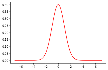
Fig. 5.18 Normal distribution with mean $\mu =0$ and variance ${\sigma }^2=1$

Now, let’s add (in blue) a normal distribution with the same mean, but a large standard deviation ($\sigma =2$). Note how it is centered at the same place as the previous normal, but more “spread out”, in line with its larger variance.

Fig. 5.19 A second normal distribution in blue with mean $\mu =0$ and standard deviation $\sigma =2$

Finally, we will add (in green) another normal, with a standard deviation of 2, but with a mean of 2. Note how it shifts up the $x$-axis, but looks otherwise similar to the blue one.

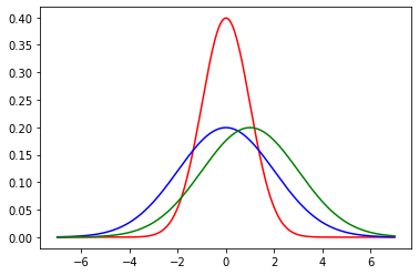
Fig. 5.20 A third normal distribution in green with mean $\mu =2$ and standard deviation $\sigma =2$

For convenience, a particular normal is sometimes written as $\mathcal{N}(\mu ,{\sigma }^2)$ or $\mathcal{N}(\mu ,\sigma )$ depending on whether you are giving the variance or standard deviation. So, for example, our green distribution might be rendered as $\mathcal{N}(2,4)$ (in the variance case) or $\mathcal{N}(2,2)$ (in the standard deviation case).

As we hinted above, many many things are normally distributed in nature, like human heights or birth weights.

Features of the normal: the “empirical rule”

The symmetry of the normal distribution, along with some other important features, leads to the Empirical Rule. This rule states that if a variable is normally distributed…

• approximately 68% of the observations will be between one standard deviation above and below the mean…

• approximately 95% of the observations will be between two standard deviations above and below the mean…

• approximately 99% of the observations will be between three standard deviations above and below the mean.

This rule is shown graphically below:

Fig. 5.21 Empirical rule

To understand the Empirical Rule, notice that the mean ($\mu$) and standard deviation ($\sigma$) are just numbers. They take particular values, and so writing $\mu +2\sigma$ literally means “the value of the mean plus the value of two times the value of the standard deviation”.

To give an example, suppose we have women’s heights, which we believe to be normally distributed. The mean of those heights is $\mu =65$ inches. The standard deviation is $\sigma =3.5$ inches. What does the Empirical Rule say?

It says:

• approximately 68% of the observations will be between one standard deviation above and below the mean…

Well, one standard deviation above the mean is $65+3.5=68.5$ (we just add one standard deviation value to the mean value); one standard deviation below the mean is $65-3.5=61.5$ (we just subtract one standard deviation value from the mean value). So: approximately 68% of all women have heights between 61.5 and 68.5 inches. Next:

• approximately 95% of the observations will be between two standard deviations above and below the mean…

Well, two standard deviations above the mean is $65+(2\times 3.5)=72$ (we just add two standard deviations to the mean value); two standard deviations below the mean is $65-(2\times 3.5)=58$ (we just subtract two standard deviations from the mean value). So: approximately 95% of all women have heights between 58 and 72 inches. Next:

• approximately 99% of the observations will be between three standard deviations above and below the mean.

Well, three standard deviations above the mean is $65+(3\times 3.5)=75.5$ (we just add three standard deviations to the mean value); three standard deviations below the mean is $65-(3\times 3.5)=54.4$ (we just subtract three standard deviations from the mean value). So: approximately 99% of all women have heights between 54.4 and 75.5 inches.

In a sense, it is not surprising that almost all women’s heights are between 4 foot 6 and a half inches and almost six foot, four inches. But this is nonetheless quite informative about how a variable is distributed, how likely we are to see a case above or below a certain point, and so on.

$Z$-Scores

We can make the idea of the Empirical Rule more general. Rather than focusing on “whole numbers” of standard deviations (so, 1 or 2 or 3), we can give every observation a score in terms of where it lies relative to the mean of the normal distribution from which it was drawn.

We will define the $Z$-Score of an observation as

the value of the observation minus the mean of the distribution, divided by the standard deviation of the distribution.

That is:

$$Z=\frac{X-\mu }{\sigma }$$

where:

• $X$ is the value of the observation (the specific height, or weight, or income or whatever)

• $\mu$ is the value of the mean of the normal distribution from which it is drawn

• $\sigma$ is the value of the standard deviation of the normal distribution from which it is drawn

The intuition is that, but converting the observation to a $Z$-Score, we are putting it in terms of “standard deviations away from the mean”. If the $Z$-Score is positive the observation is above the mean; if the $Z$-Score is negative the observation is below the mean.

Men’s weights as $Z$-Scores

Suppose that the mean weight of a man in the US is 191 pounds ($\mu =$191 lbs). Suppose the standard deviation of weights is 43 pounds ($\sigma =$43 lbs). Consider three observations (people) and their weights:

1. 176 lbs. Then: $Z=\frac{176-191}{43}=-0.34$

2. 302 lbs. Then: $Z=\frac{302-191}{43}=2.58$

3. 80 lbs. Then: $Z=\frac{80-191}{43}=-2.58$

Notice that the second (302 lbs) and third (80 lbs) men were equally far from the mean, but above and below it respectively—in both cases, they are 2.58 standard deviations away.

Standard Normal

When we subtract the mean and divide by the standard deviation, we are standardizing our distribution. Whatever normal distribution we start with, whatever its mean and variance, we will end up with a normal distribution that has:

• mean equal to zero ($\mu =0$)

• standard deviation (and variance) equal to one ($\sigma ={\sigma }^2=1$)

This distribution is called the standard normal, and is written as $\mathcal{N}(0,1)$. Note that there is no ambiguity as to whether the ‘1’ is for the variance or the standard deviation, because there are the same in this special case.

The standard normal look as we would expect (it is centered at zero) and, in fact, we met it already above:

Fig. 5.22 Standard normal

To reiterate: the distribution of $Z$-Scores, sometimes called the $Z$-distribution, is standard normal.

The $Z$-distribution and probabilities

Converting observations to $Z$-scores allows us to calculate probabilities of seeing units of different values. To get the intuition, recall when we showed that, based on $Z$-score, 99% of all women were between 54.4 and 75.5 inches. This immediately suggests that the proportion of women taller than 75.5 inches is very small. Another way to put this is that the probability that a woman randomly drawn from the population is taller than 75.5 inches is very small.

To make this more formal, consider the following question:

• what proportion of women are taller than 5 feet 9 inches?

This is the same as asking what proportion of women have heights in excess of 69 inches, which itself is the same as asking what the probability of a random woman being over 69 inches tall.

In $Z$-score terms, 69 inches is

$$Z=\frac{65-69}{3.5}=1.14$$

So we want to know the probability of observing $Z>1.14$ for a random woman in the population.

To understand this problem graphically, consider the following figure:

Fig. 5.23 Observation with $Z=1.14$

We have an observation with $Z=1.14$. That’s a little above the mean, as we see on the figure. We want to know what proportion of the distribution is larger than this value. This is equivalent to asking about the size of the blue colored area is: from the $Z=1.14$ point out to infinity.

To calculate this, we can ask Python “for a standard normal distribution, what is the size of the area to the right of $Z=1.14$?” In practice, we do this by asking a more roundabout question: “what is the size of the total distribution minus the area that begins 1.14 standard deviations below the mean?” To do this, we need a function norm.cdf from stats in scipy:

from scipy import stats
1-stats.norm.cdf(1.14)

0.12714315056279824

The “1” here captures the fact that all distributions sum to one (the probability of observing all the possible heights must be one in total). We subtract the 1.14 to tell us how much of the distribution remains once we remove those folks below that height.

This comes out to a probability of around 0.127; equivalently, that 12.7% of women are taller than 5’9”.

Let’s consider a different problem. Suppose we want to know what proportion of women are under 5’3”. This is equivalent to asking what proportion of women have a $Z$-Score less than $\frac{63-65}{3.5}=-0.57$. And that is equivalent to asking what proportion of the height distribution is shaded blue in this figure:

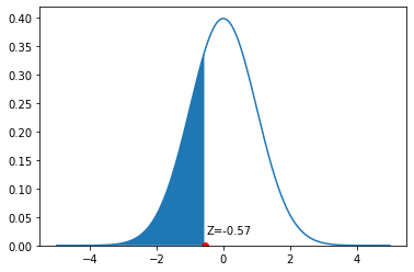
Fig. 5.24 Observation with $Z=-0.57$

Now, we can simply ask for:

stats.norm.cdf(-.57)

0.28433884904632417

This works, because norm.cdf is set up to tell us what proportion of the distribution is below the argument we gave it (a $Z=-0.57$). And it is around 0.28: the probability of a random women having a height less than or equal to 5’3” is 0.28. It immediately follows the proportion of women taller than 5’3” is 1-0.28=0.72. That is the entire area to the right of the blue color.

Finally, suppose we want to know the proportion of observations between two values. Let’s say, the proportion of women between 5’4” and 5’8”. We need the proportion of the normal between a $Z$-Score of $\frac{64-65}{3.5}=-0.28$ and $\frac{68-65}{3.5}=0.86$. On the density, this is the blue area pictured:

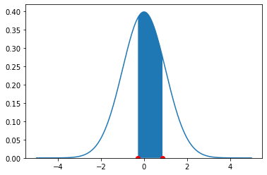
Fig. 5.25 Observations with $-0.28\ge Z\le 0.86$

There are several different ways to proceed here. Perhaps the simplest is to request the area above the higher number (so, $>0.86$), then request the area below the lower number (so, $<-0.28$) and then subtract both areas from 1. Hence:

1- (1- stats.norm.cdf(0.86) ) - stats.norm.cdf(-0.28)

0.4153667263039888

Or around 41.4%. This implies that a random draw will select a woman between 5’4” and 5’8” with probability 0.415.