Population parameters and sample statistics
Contents
4.2. Population parameters and sample statistics#
Before we get into the materials, it will be helpful to load some libraries so you can replicate the plots and other code below.
#let's import numpy,
import numpy as np
# and matplotlib
import matplotlib.pyplot as plots
# and we'll use pandas briefly too
import pandas as pd
In most statistical reasoning problems, we are trying to make an inference about a population. The population is the
universe of cases we wish to describe.
It is easy to think of examples of questions that require us to learn something about a population:
How will every voter (who turns out to vote) vote in the United States in the 2024 Presidential election? This is something opinion polls try to estimate.
What is the average income (per household) in the United Kingdom? We might want to estimate this, so we can compare the UK to other countries, or for policy-making.
What proportion of the people living in NYC have been a victim of crime this year?
How common is a particular animal species (say, the red fox) in the world? is it becoming more or less numerous over time?
How polluted is the Hudson River, on average, over its length?
We call the characteristic we care about—the vote choice, the proportion who have had COVID, the number of living animals from a species—the population parameter. Unfortunately, unless we do a census—where we record the status of every single member of the population—we cannot study the population directly. This may be because it is simply too time consuming, or too expensive to get that information (imagine asking every single one of the 200 million voters who they expect to cast their ballots for, or trying to survey every inch of the world to count up how many red foxes live there).
Consequently we will often resort to using a sample to make inference about the population. Specifically, we will use sample statistics to estimate population parameters. The use of the term “estimate” here is important: because we will not generally have access to the whole population, we can never know the population parameter value with absolute certainty. But we will be able to talk about our estimates of those parameters and the uncertainty around them.
In this course, we will mostly focus on large, random samples. This is in keeping with the sorts of datasets many data scientists find they have access to in the real world. In more traditional social science courses, one often has very small samples (< 30), which calls for some special techniques we will not cover.
Random Samples#
When we talk about a sample being random we mean
the units in the sample are selected in a non-deterministic way, by chance
We will give more details, and examples, below. For now, by “non-deterministic” we mean that if we did the sampling all over again, we would expect it to come out differently—that is, the units (people, voters etc) we would draw would be different.
We met the idea of “random sampling” before, when we talked about randomized control trials. There, we wanted to randomize people to treatment or control. This was motivated by wanting to avoid the subjects self-selecting into a particular group; by extension this would eliminate potential biases or differences between the groups in terms of background characteristics.
There is a similar idea here, insofar as we don’t want particular types of units disproportionately ending up in the sample we use. Fortunately, computers are extremely good at generating all things random, including random numbers and random samples. So we will use them.
Probability Samples#
For a probability sample
before we draw the sample, we can calculate the chance that any given unit (from the population) will appear in the sample
The most famous and obvious example is a simple random sample (sometimes “SRS”, sometimes “\(\frac{1}{n}\) sampling”) where
the probability of any given unit appearing in the sample is \(\frac{1}{n}\), where \(n\) is the size of the sample.
Some simple examples can help fix ideas:
suppose we are randomly drawing balls for a draft lottery, and each ball has a day of the year on it. Ignoring leap years, the probability that we draw a given date, say September 9 is \(\frac{1}{365}\) or around 0.0027.
suppose we are randomly drawing cards from a regular deck. The probability of drawing a King is \(\frac{4}{52}\) or around 0.077.
Sampling with and without replacement#
Returning to the draft lottery idea, recall that each ball (if we ignore leap years) has a probability of \(\frac{1}{365}\) of being selected. Suppose I sample one ball (one date). I could then:
replace it, meaning I just put it back with the others balls. Now the chance of picking any given date is, once again, \(\frac{1}{365}\). This is called sampling with replacement.
not replace it, meaning I remove it from all the other balls permanently. Now the chance of picking any remaining date ball in the lottery is \(\frac{1}{364}\), and the probability of me picking the ball I already picked is zero. This is called sampling without replacement.
We can simulate this difference with basic code. First, we will define an object call days: it is just all the numbered balls in the lottery (there are 365 of them, but this needs to be set up as a range from 1 through 366).
days = np.arange(1,366)
Let’s draw a sample of size 100 with replacement (replace=True):
days_draw_replace = np.sort(np.random.choice(a= days, size =100,
                                             replace = True))
If you take a look at days_draw_replace you should see some repeat days (why?). Let’s draw without replacement:
days_draw_noreplace = np.sort(np.random.choice(a= days, size =100,
                                               replace = False))
If you look at days_draw_noreplace you will see that, now, there are no repeats (why?).
Probability Distributions#
Let’s start with a simple experiment. We will roll one “fair” (think: unbiased) six-sided die, and see how it comes up: i.e. what numbers we roll. What percentage of the time do we think it will come up “1” v “2” v “3” etc? Let’s plot all the values it could take, and the percentage of the time we expect each outcome. We will call this the probability distribution: it is how the data should stack up. It will look something like this:
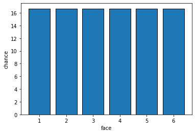
Fig. 4.1 Probability distribution of outcomes for one fair die#
Each face should be rolled about \(\frac{100}{6}\) of the time. Which is somewhere around 17%. Notice that here, each possible outcome is in a separate ‘bin’—we cannot roll 5.5 or 3.234 etc. So we say this distribution is discrete. Second, you can see that all the faces are as likely as each other. We use the term uniform to describe such distributions. So: this is a discrete uniform distribution.
Now this is how we expect the die to behave. What will happen in a specific set of rolls that we do is called the empirical distribution.