10.6. Predicting continuous outcomes#

Until now, we have been interested in predicting categories for observations. But it will often be the case that we want to predict continuous numerical outcomes like incomes, prices or temperatures. We can use the tools we have already learned about—linear regression and $kNN$—to do this.

import matplotlib.pyplot as plt
import numpy as np
import math
import scipy.stats as stats
import statsmodels.api as sm 
import pandas as pd

Multiple regression#

Previously, we discussed regression in the context of fitting models of this type:

\[ Y = a + bX \]

where $Y$ was the outcome, $a$ was our intercept or constant, and $b$ was our slope coefficient. In that case, we had one predictor or $X$ variable. We extend that now to multiple predictors:

\[ Y = a +b_1X_1 + b_2X_2 + \ldots + b_kX_k \]

Here, $X_1$ is our first variable, $X_2$ is a second, all the way through to $X_k$ (our $k$th variable). Notice that each variable has its own slope coefficient: its own $b$. Note also terminology: we sometimes refer to the $X$ variables as the “right hand side”, because they are on the on right hand side of the equals sign. We sometimes refer to the dependent variable, the $Y$ variable, as the left hand side (for obvious related reasons).

To see how multiple (linear) regression works, we will try to predict house prices in a well-known data set.

Predicting house prices#

Our data is from Ames, Iowa. Each observation in the data set is a property for which we have a sales price. It is this sales price that we wish to predict. We will base that prediction on the $X$ variables available to us, which are extensive. They include the size of the first floor, the size of basement, the size of the garage area, the year the house was built and so on. It seems reasonable to believe we would want to include many (or all) of these variables in our predictions, and multiple regression with allow for that.

Let’s pull in the data. Our interest will be in one family homes (1Fam) that are in normal condition, so we will restrict the data to those. In addition, we will restrict our models to a subset of all the predictors available, mostly just to simplify the presentation.

all_sales = pd.read_csv('data/house.csv')
fam_sales = all_sales[all_sales['Bldg.Type']=="1Fam"]
norm_fam = fam_sales[fam_sales['Sale.Condition']=="Normal"]

sales = norm_fam[['SalePrice', 'X1st.Flr.SF', 'X2nd.Flr.SF',
                  'Total.Bsmt.SF', 'Garage.Area',  'Wood.Deck.SF', 
                  'Open.Porch.SF', 'Lot.Area',
                       'Year.Built', 'Yr.Sold']]

We can take a quick look at the data; here we sort from cheapest to most expensive, and take the ‘top’ 4:

sales.sort_values(by='SalePrice').head(4)

	SalePrice	X1st.Flr.SF	X2nd.Flr.SF	Total.Bsmt.SF	Garage.Area	Open.Porch.SF	Lot.Area	Year.Built	Yr.Sold
2843	35000	498	0	498.0	216.0	0	8088	1922	2006
1901	39300	334	0	0.0	0.0	0	5000	1946	2007
1555	40000	649	668	649.0	250.0	54	8500	1920	2008
708	45000	612	0	0.0	308.0	0	5925	1940	2009

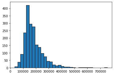
Typically, prices of properties are right skewed: the mean property is much more expensive than the median one. That seems to be the case here, too:

plt.hist(sales['SalePrice'], bins=32, ec="black")
plt.show()

../../_images/05_continuous_outcomes_8_0.png

Working with the data: training/test split#

As usual with prediction problems, we will split the data, and learn the relationship between $X$ and $Y$ in the training set. We will then see how well we predict the outcomes in the test set. In particular, we will:

split the data evenly and randomly into training and test set
fit a multiple linear regression to the training set that models $Y$ in the training set as a function of the $X$s in the training set
Use the model results from the training set (for us, the estimated coefficients) to predict the $Y$ in the test set (based on the $X$s in the test set)
Compare our predictions (the fitted values) with the actual sales prices in the test set to get a sense of how well our model performs

As previously, we form the training set by sampling without replacement from the data. Then, anything we do not use in training goes to the test set. We do this telling Python to drop the observations assigned to train from the original data set and make the residual data the test set. We will set a random_state again, just to ensure everyone gets the same results.

train = sales.sample(frac=0.5, replace=False, random_state=5) 
test  = sales.drop(train.index)

print(len(train), 'training and', len(test), 'test instances.')

1001 training and 1001 test instances.

Working with multiple regression#

Previously, when we conducting a linear regression—e.g. regressing the percentage of a state’s population that smokes on the cigarette tax—we had one $Y$ variable and one $X$ variable. Perhaps somewhat confusingly, this set up is called a bivariate regression. We interpreted a given slope coefficient (the $b$ or $\hat{\beta}$) as

the (average) effect on $Y$ of a one unit change in $X$

Now we have a multiple regression which involves one $Y$ (still), but many $X$s. As a side-note, this is not a “multivariate” regression, which describes something else. In any case, a given estimated $b$ tells us

the (average) effect on $Y$ of a one unit change in that $X$, holding the other variables constant

Implicitly, this is allowing us to compare like with like: when we talk of the effect of, say, size of the first floor on the sales price ($Y$), it is as if we are comparing houses which have the same size second floor, the same size garage and so on. We are then asking “what would happen to these similar houses (in terms of their price, on average) if we altered this one factor?”

Working with Python#

As always, there are many ways to estimate a given model. We will use the statsmodel.api module, and within that the OLS function. Recall that OLS stands for “ordinary least squares”, and is the fitting method for the regression.

The constant term#

One thing to be aware of is that not all packages fit an intercept term (also called the constant) by default. That is, instead of fitting this model:

\[ Y = a +b_1X_1 + b_2X_2 + \ldots + b_kX_k \]

They fit:

\[ Y = b_1X_1 + b_2X_2 + \ldots + b_kX_k \]

where the $b$s adjust for the fact that there is no $a$ coefficient.

This behavior is the case for the OLS function. For a prediction problem like ours below, it won’t make a lot of difference practically. Still, it’s worth thinking through the theory here. One argument for not including an intercept is that, for your particular problem, when all the $X$s are zero, you expect the outcome to be zero. That is perhaps plausible in the case of house prices (though it’s hard to think sensibly about a house with zero floor space). It is probably not plausible in the case of the smoking example we did.

In any case, it is easy to add a constant, and we will do so in what follows below. We suggest you always do that, unless explicitly instructed otherwise.

Fitting to the training data#

Recall we fit the regression to the training data (the training $X$ and $Y$), learn the $b$ coefficients there, and see how well it predicts the test set.

First, we define what we want our outcome and predictors to be:

y = train[["SalePrice"]]
X = train[['X1st.Flr.SF', 
              'X2nd.Flr.SF','Total.Bsmt.SF',"Garage.Area",
           "Wood.Deck.SF","Open.Porch.SF",
              "Lot.Area","Year.Built","Yr.Sold"]]

Now we fit the model (via a fit() call), explicitly telling Python to add_constant to the $X$ values first:

Xc = sm.add_constant(X.values)
est = sm.OLS(y, Xc).fit()

Although it does not matter for prediction, a slightly annoying feature of this set up is that it losses the variable names when one asks for the results. We can fix that just by setting the xname argument of the model when we ask for a summary. First, we define the coefficient names: these are just the constant followed by the variable names (which we get from the columns of X, above). We make everything into a list, and pass that to xname.

xcol_names  = X.columns
coefficient_names = list( xcol_names.insert(0,"constant") )

We now request the summary:

est.summary(xname = coefficient_names)

OLS Regression Results
Dep. Variable:	SalePrice	R-squared:	0.819
Model:	OLS	Adj. R-squared:	0.817
Method:	Least Squares	F-statistic:	497.0
Date:	Thu, 25 Aug 2022	Prob (F-statistic):	0.00
Time:	15:16:53	Log-Likelihood:	-11788.
No. Observations:	1001	AIC:	2.360e+04
Df Residuals:	991	BIC:	2.364e+04
Df Model:	9
Covariance Type:	nonrobust

	coef	std err	t	P>\|t\|	[0.025	0.975]
constant	-1.815e+06	1.57e+06	-1.160	0.246	-4.89e+06	1.26e+06
X1st.Flr.SF	79.5697	4.905	16.222	0.000	69.944	89.195
X2nd.Flr.SF	74.7584	2.658	28.127	0.000	69.543	79.974
Total.Bsmt.SF	40.7796	4.170	9.778	0.000	32.596	48.963
Garage.Area	48.9083	6.316	7.744	0.000	36.514	61.302
Wood.Deck.SF	42.5366	8.385	5.073	0.000	26.082	58.991
Open.Porch.SF	30.2960	16.094	1.882	0.060	-1.286	61.878
Lot.Area	0.6534	0.148	4.414	0.000	0.363	0.944
Year.Built	538.0643	41.121	13.085	0.000	457.370	618.759
Yr.Sold	369.7964	779.627	0.474	0.635	-1160.112	1899.705

Omnibus:	248.060	Durbin-Watson:	1.998
Prob(Omnibus):	0.000	Jarque-Bera (JB):	1419.273
Skew:	1.007	Prob(JB):	6.44e-309
Kurtosis:	8.474	Cond. No.	2.06e+07

Warnings:
[1] Standard Errors assume that the covariance matrix of the errors is correctly specified.
[2] The condition number is large, 2.06e+07. This might indicate that there are
strong multicollinearity or other numerical problems.

Each element of coef in the table is a coefficient. These are the slope estimates. So, for example, the $b$ on Garage.Area is 48.9. This tells us that, holding all other variables constant, a one square foot increase in the garage area of a house is expected to increase the sale price by $48.90 (on average).

The P>|t| gives the $p$-value for each coefficient. And we see there is also (top right) $R$-squared should we want it.

But to reiterate, we are not particularly interested in interpreting the coefficients here: they are helpful to the extent they aid prediction.

Making Predictions with Multiple Regression#

With bivariate regressions, if you gave me an $X$ value, I could immediately predict a $Y$ ($\hat{Y}$) value by just plugging that $X$ value into the equation, and multiplying by the $b$ estimate and adding the $a$ estimate to that product.

The story with multiple regression is very similar. Now though we produce

\[ \hat{Y} = a+b_1x_1+b_2x_2+\ldots+b_kx_k \]

That is, we predict a $Y$-value for the observation by taking the observation’s value on $x_1$ (X1st.Flr.SF) and multiplying that by our $b_1$ estimate (79.57) and adding it to the observation’s value on $x_2$ (X2nd.Flr.SF) and multiplying that by our $b_2$ estimate (74.76) and so on through all the variables down to the observation’s Yr.sold multiplied by that coefficient (369.80). Finally we add the constant to this.

We want to take this prediction machinery to the test set. We use the model from the training set (the coefficients) and multiple them by the $X$ values in the test set. Thus we will obtain a predicted $Y$ (a $\hat{Y}$) for every observation in the test set.

But we also have the actual values of the $Y$ in the test set. If we have done a good job of modeling, our predicted $Y$s should be similar to the true Ys in the test set.

So, we need to create our test set $X$s, and add a constant (to make it comparable to the model above). Then we use the model we fit to the training set (called est) to make predictions based on that model but with the “new” data (the test set). We use the .predict function for this:

X_test = test[['X1st.Flr.SF', 'X2nd.Flr.SF','Total.Bsmt.SF',
               "Garage.Area","Wood.Deck.SF","Open.Porch.SF",
               "Lot.Area","Year.Built","Yr.Sold"]]
Xnew = sm.add_constant(X_test.values) 

ynew =  est.predict(Xnew) 

Are our predictions good? If they were perfect, we would expect that our $\hat{Y}$ for the test set would be identical to the true Y values for the test set, observation by observation. But if that is the case, we would expect all the actual $Y$s and prediction $Y$s to line up on a 45 degree line. Let’s see:

plt.scatter(ynew, test[['SalePrice']], edgecolor="black")
plt.ylabel("actual (test) data")
plt.xlabel("fitted")
plt.xlim(0, 500000)
plt.ylim(0,500000)
plt.plot([-100, 5e5], [-100, 5e5], color="black")
plt.show()

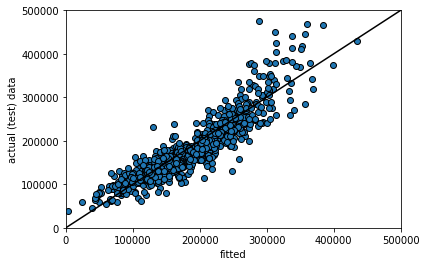
../../_images/05_continuous_outcomes_26_0.png

Here ynew is our prediction for the test set (the fitted values, $\hat{Y}$); the actual $Y$ is our actual sales prices from the test set. Generally, these line up fairly well. Clearly, as the true price gets higher, we tend to predict higher prices. That said, In particular, we seem to under-predict the actual values at medium-high (true) sales prices. For example, we predict a whole bunch of houses to be $ \$300-400k$, which were actually sold for price around $\$400-500k$. It seems that it is generally harder to predict the very high price sales.

Nearest Neighbor regression#

Multiple regression is not the only way to work with continuous outcomes. Another option is to use our nearest neighbor ideas from before. Obviously, we won’t be taking a “vote” anymore, because the outcomes are not categories. Instead, we will find the $k$ nearest neighbors and take the mean. This will be our prediction for the test set.

More specifically, to predict a value for a test set observation, we simply find the $k$ nearest neighbors in the training set (in terms of the $X$s relative to our test set observation), and take the average of their outcomes.

To do this, we need functions similar to those we wrote before. With some minor changes we can produce a predictor of continuous outcomes.

def distance(pt1, pt2):
    """The distance between two points, represented as arrays."""
    return np.sqrt(sum((pt1 - pt2) ** 2))

def row_distance(row1, row2):
    """The distance between two rows of a table."""
    return distance(np.array(row1), np.array(row2))

def distances(training, example, output):
    """Compute the distance from example for each row in training."""
    dists = np.array([])
    attributes = training.drop(output, axis=1)
    for row in np.arange(len(attributes)):
        dists = np.append(dists, row_distance(attributes.iloc[row,],
                                              example))
    training2 = training.copy(deep=True)
    training2["Distance"] = dists
    return training2

def closest(training, example, k, output):
    """Return a table of the k closest neighbors to example."""
    dista = distances(training, example, output)
    sort_dist = dista.sort_values(by="Distance")
    sort_dist_top = sort_dist.take(np.arange(k), axis=0)
    return sort_dist_top

These four functions:

take a Euclidean distance between two points (distance)
allow one to take this distance for rows of data (i.e. attributes) (row_distance)
produce a distance for an observation from every row of the data (distances)
return the $k$ rows in the data with the shortest distances from the point in question (closest)

The prediction will be based on those $k$ closest rows, and involves taking the mean—the np.average()—of the $k$ outcomes. This function will do that:

def predict_nn(example):
    """Return the average Y among the k nearest neighbors."""
    return np.average(closest(train, example, 5, 'SalePrice')['SalePrice'])

As written, this function passes the requisite $k$ (5 here) directly to closest(), and it also specifies the outcome of interest SalesPrice.

We can apply this to our data, by first creating a test set of attributes only. Note that this code takes a little while to run ($\sim2$ minutes).

test_df = test.drop('SalePrice', axis=1)

nn_test_predictions= test_df.apply(predict_nn, axis=1)

In principle, we can just compare our “true” values of the sales price with our $kNN$ predictions. So, something like:

kpred = {'knn prediction': nn_test_predictions}
table_comparecont = pd.DataFrame(kpred)
table_comparecont["actual value"] = test["SalePrice"]
table_comparecont.head()

	knn prediction	actual value
0	169800.0	215000
5	190800.0	195500
12	175800.0	180400
13	182900.0	171500
19	269280.0	210000

But we would like something more systematic, and that allows us to compare this model’s performance with that of the multiple regression.

Root Mean Square Error#

Root Mean Square Error (RMSE) is a popular way to compare models, and also to get an absolute sense of how well a given model fits the data. We define each term in turn:

error is the difference between the actual $Y$ and the predicted $Y$ and is $( \mbox{actual } Y- \hat{Y})$. Ideally we would like this to be zero: that would imply our predictions were exactly where they should be.
square simply means we square the error. We do this for reasons we met above in other circumstances: if we don’t square the error, negative and positive ones will cancel out, making the model appear much better than it really is. This is $( \mbox{actual } Y- \hat{Y}) ^2$
mean is the average. We want to know how far off we are from the truth, on average. This is $\frac{1}{n}\sum ( \mbox{actual } Y- \hat{Y}) ^2$
root simply means we take the square root of the squared error. We do this to convert everything back to the underlying units of the $Y$ variable.

Thus, RMSE is

\[ = \sqrt{\frac{1}{n}\sum ( \mbox{actual } Y- \hat{Y})^2} \]

Note that this quantity is sometimes known as the Root Mean Square Deviation, too.

Features of RMSE#

Clearly, a lower RMSE is better than a higher one. The key moving part is the difference between the prediction for $Y$ and the actual $Y$. If that is zero, the model is doing as well as it possibly can.

The size of the RMSE is proportional to the squared error. That is, it is proportional to $( \mbox{actual } Y- \hat{Y})^2$. This means that larger errors are disproportionately costly for RMSE. For example, from the perspective of RMSE it is (much) better to have three small errors of 2 each (meaning $2^2+2^2+2^2=12$) rather than, say, one error of 1, one of zero and one of 5 (meaning $1^2+0+5^2=26$). This is true even though the total difference between the actual and predicted $Y$ is 6 units in both cases.

A related metric you may see in applied work is the Mean Absolute Error (MAE). This $\frac{1}{n}\sum | \mbox{actual } Y- \hat{Y}| $. The $|\cdot|$ bars tell you to take the absolute value of what is inside them. Like the RMSE, MAE is on the same underlying scale as the data. Unlike the RMSE, however, the MAE does not punish bigger errors disproportionately more (but it does punish them more).

Intuitively, the RMSE tells us

on average, based on the attributes, how far off the model was from the outcomes in the test set.

RMSE in Practice#

Despite the long description, the code to calculate the RMSE is simple. We first calculate the square of the difference of every predicted $Y$-value relative to every actual test set $Y$ value, and take the average (np.mean) of those. Then we take the square root of that quantity.

For the multiple regression we have:

MSE_regression = np.mean((ynew - test['SalePrice'])**2) 
RMSE_regression = MSE_regression**(.5)

print("\n the regression RMSE was:",
      RMSE_regression,"dollars")

 the regression RMSE was: 30833.875818953995 dollars

So the multiple regression was about $\$31$k dollars off (on average) for each predicted sales price. What about the $kNN$ regression?

rmse_nn = np.mean((test["SalePrice"] - nn_test_predictions) ** 2) ** 0.5
print("\n RMSE of the NN model is:", rmse_nn, "dollars")

 RMSE of the NN model is: 43862.09151710011 dollars

For the $kNN$ model it is a little higher, missing the actual value by about $\$44$k dollars on average. For this problem then, we would conclude the multiple regression was the better model.

Aside: using `Scikit-learn` for NN regression#

Just for completeness, we show that we can replicate our results above with Scikit-learn. First we import the relevant module and initialize the regression (we tell the module the number of nearest neighbors):

from sklearn.neighbors import KNeighborsRegressor
knnr = KNeighborsRegressor(n_neighbors=5)

We then set up the training and test sets, making sure to properly assign the outcome and the predictors, and fit the regression model using fit():

X_train = train.drop(["SalePrice"], axis=1)
X_test = test.drop(["SalePrice"], axis=1)
Y_train = train["SalePrice"]
Y_test = test["SalePrice"]

knnr.fit(X_train, Y_train)

KNeighborsRegressor(algorithm='auto', leaf_size=30, metric='minkowski',
                    metric_params=None, n_jobs=None, n_neighbors=5, p=2,
                    weights='uniform')

We then give the model the $X$s from the test set and tell it to predict $Y$ values based on this:

y_pred = knnr.predict(X_test)

Finally we return the RMSE after importing the relevant module from Scikit-learn:

from sklearn.metrics import mean_squared_error
print("RMSE of kNN regression from sklearn is...")
print(mean_squared_error(Y_test,y_pred)**(.5)) 

RMSE of kNN regression from sklearn is...
43862.09151710011

Additional aside: when to use $kNN$ vs. multiple regression#

Above, we showed that multiple regression performed a little better overall for predicting house sales prices. But, of course, we should not always expect this to be true. There is a big literature on anticipating what types of models do better on what types of data, and we will not try to summarize that here. Nonetheless, it is worth noting by its very nature $kNN$ tends to do better when there are non-linear relationships in the data. This is because $kNN$ uses points ‘local’ to the given observation to make predictions, and this allows the relationships between the $X$s and the $Y$s to be quite different for different values of $X$. Whereas something like a linear regression does not allow this.

To get a sense of this, let’s make a toy data set. We will have a $Y$ variable which is the sales price of houses again, but this time our (one) $X$ variable is distance to the nearest train station. In general, we anticipate that being near the train station leads to a higher price (because people commute). But as we get very close to the train station, we expect prices to decline. This is because public transit stops can be noisy, attract traffic etc.

miles_from_station = np.arange(.2, 3, .01)

Here miles_from_station goes from a low number (0.2 miles, so about a five minute walk) to a high number (3 miles, which one would need to drive or cycle presumably). We will suppose that prices are a non-linear function of this distance.

prices = 500000 - ((1.5-miles_from_station)*400)**2 
actual_ps = prices + np.random.normal(loc=0, scale=40000, 
                                      size=len(prices))

Here, prices are a quadratic function of the distance from the station. They are maximized at 1.5 miles away: so walkable, but not too close in terms of the downsides of too short a distance. To construct actual_ps we just add some random noise to the prices to reflect the idea that markets aren’t perfect and things are measured with error etc.

If we plot the data, the pattern is clear:

plt.scatter(miles_from_station, actual_ps, ec="black")
plt.ylabel("price")
plt.xlabel("distance from station")
plt.show()

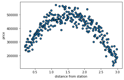
../../_images/05_continuous_outcomes_60_0.png

Basically, a house close or far from the station is the cheapest option. One that is an “ideal” distance (1.5 miles) is the most expensive.

Let’s set up a training and and test set, and see how multiple regression versus $kNN$ regression does on this problem. First we will put everything in a data frame.

the_data = pd.DataFrame({'house_price': actual_ps, 
                         'miles': miles_from_station})

train_data = the_data.sample(frac=0.5, replace=False, random_state=6)
test_data  = the_data.drop(train_data.index)

Regression model#

Now we fit the regression model:

yp = train_data[['house_price']]
Xp = sm.add_constant(train_data[['miles']].values)
estp = sm.OLS(yp, Xp).fit()

Now predict the test set:

Xp_test = test_data[['miles']]
Xpnew = sm.add_constant(Xp_test.values) 
ypnew =  estp.predict(Xpnew) 

And report the RMSE:

pMSE_regression = np.mean((ypnew - test_data['house_price'])**2) 
pRMSE_regression = pMSE_regression**(.5)

print("\n the regression RMSE was:",
      pRMSE_regression,"dollars")

 the regression RMSE was: 98008.42561004696 dollars

So each prediction for the regression is about $\$100$k dollars off, on average.

$kNN$ comparison#

Now we will do the same thing, but for the $kNN$ regression:

knnp = KNeighborsRegressor(n_neighbors=5)

Xp_train = train_data.drop(["house_price"], axis=1)
Xp_test = test_data.drop(["house_price"], axis=1)
Yp_train = train_data["house_price"]
Yp_test = test_data["house_price"]

knnp.fit(Xp_train, Yp_train)
yp_pred = knnp.predict(Xp_test)
print(mean_squared_error(Yp_test,yp_pred)**(.5)) 

41273.296025093405

Here, each prediction is about $\$44$k dollars off. This is a large improvement over the linear regression. And that makes sense: a linear model is the wrong choice for an obviously non-linear relationship.

Data Science for Everyone

Predicting continuous outcomes

Contents

10.6. Predicting continuous outcomes#

Multiple regression#

Predicting house prices#

Working with the data: training/test split#

Working with multiple regression#

Working with Python#

The constant term#

Fitting to the training data#

Making Predictions with Multiple Regression#

Nearest Neighbor regression#

Root Mean Square Error#

Features of RMSE#

RMSE in Practice#

Aside: using `Scikit-learn` for NN regression#

Additional aside: when to use \(kNN\) vs. multiple regression#

Regression model#

\(kNN\) comparison#

Data Science for Everyone

Predicting continuous outcomes

Contents

10.6. Predicting continuous outcomes#

Multiple regression#

Predicting house prices#

Working with the data: training/test split#

Working with multiple regression#

Working with Python#

The constant term#

Fitting to the training data#

Making Predictions with Multiple Regression#

Nearest Neighbor regression#

Root Mean Square Error#

Features of RMSE#

RMSE in Practice#

Aside: using Scikit-learn for NN regression#

Additional aside: when to use \(kNN\) vs. multiple regression#

Regression model#

\(kNN\) comparison#

Aside: using `Scikit-learn` for NN regression#